Chapter 2: Time Series Data
Introduction
Since the advent of Relational Database Technology, many new requirements to manage data have emerged. Luminaries, such as Martin Fowler, have proposed Polyglot Persistence1 as one solution for managing diverse data and data processing requirements.
However, Polyglot Persistence comes with costs and has attracted criticisms, such as2:
In an often-cited post on polyglot persistence, Martin Fowler sketches a web application for a hypothetical retailer that uses each of Riak, Neo4j, MongoDB, Cassandra, and an RDBMS for distinct data sets. It’s not hard to imagine his retailer’s DevOps engineers quitting in droves.
— Stephen Pimentel
and also3:
What I’ve seen in the past has been is if you try to take on six of these [technologies], you need a staff of 18 people minimum just to operate the storage side - say, six storage technologies. That’s not scalable and it’s too expensive.
— Dave McCrory
There have also been some proposals for using micro-services to implement a Polyglot Persistence architecture in recent years4. However, SingleStore can provide a simpler solution by supporting diverse data types and processing requirements in a single multi-model database system. This offers many benefits, such as lower Total Cost of Ownership (TCO), less burden upon developers to learn multiple products, no integration pains and more. In this and the following chapters, we’ll discuss SingleStore’s multi-model capabilities in greater detail. We’ll start with Time Series data.
We’ll use historical S&P 500 stock data from Kaggle5 licensed under CC0 1.0, allowing unrestricted use, including for commercial purposes. We’ll also build a quick dashboard to visualize candlestick charts using Streamlit.
The dataset consists of the following fields:
-
date: Spans a five-year daily period from 8 February 2013 until 7 February 2018. No missing values.
-
open: Opening price. 11 missing values.
-
high: High price. 8 missing values.
-
low: Low price. 8 missing values.
-
close: Closing price. No missing values.
-
volume: Total shares traded. No missing values.
-
Name: Trading symbol. 505 unique values. No missing values.
For our initial exploration, we’ll select date, close and Name.
Create the Database and Table
In the SingleStore Portal, we’ll use the SQL Editor to create a new database. Let’s call this timeseries_db, as follows:
CREATE DATABASE IF NOT EXISTS timeseries_db;
We’ll also create a table, as follows:
USE timeseries_db;

DROP TABLE IF EXISTS tick;
CREATE TABLE IF NOT EXISTS tick (
    ts     DATETIME SERIES TIMESTAMP,
    symbol VARCHAR(5),
    price  NUMERIC(18, 4),
    KEY(ts)
);
Each row has a time-valued attribute called ts. We’ll use DATETIME rather than DATETIME(6), since we are not working with fractional seconds in this example. SERIES TIMESTAMP specifies a table column as the default timestamp. We’ll create a KEY on ts as this will allow us to efficiently filter on ranges of values.
Fill out the Notebook
Let’s now create a new Python notebook. We’ll call it data_loader_for_time_series.
We’ll create a new DataFrame, as follows:
tick_csv_url = ...

tick_df = pd.read_csv(tick_csv_url)
This reads the CSV file and creates a DataFrame called tick_df.
In the next code cell, we’ll remove incomplete rows:
tick_df = tick_df.dropna()
Next, let’s get the number of rows:
tick_df.count()
Executing this will return the value 619029.
We’ll remove some of the columns based upon our earlier decision for the initial analysis, as follows:
tick_df = tick_df.drop(columns = ["open", "high", "low", "volume"])
rename some columns:
tick_df = tick_df.rename(columns = {"date": "ts", "close": "price", "Name": "symbol"})
and sort the data:
tick_df = tick_df.sort_values(by = ["ts", "symbol"])
In the next code cell, we’ll take a look at the structure of the DataFrame:
tick_df.head()
The output should look like this:
               ts    price symbol
71611  2013-02-08  45.0800      A
0      2013-02-08  14.7500    AAL
2518   2013-02-08  78.9000    AAP
1259   2013-02-08  67.8542   AAPL
3777   2013-02-08  36.2500   ABBV
We are now ready to write the DataFrame to SingleStore. First, we’ll create a connection:
from sqlalchemy import *

db_connection = create_engine(connection_url)
Next, we’ll ensure that the table is empty:
with db_connection.begin() as conn:
    conn.execute(text("TRUNCATE TABLE tick;"))
Finally, we’ll write the DataFrame to SingleStore:
tick_df.to_sql(
    "tick",
    con = db_connection,
    if_exists = "append",
    index = False,
    chunksize = 1000
)
This will write the DataFrame to the tick table in the timeseries_db database.
Example Queries
Now that we’ve built our system, we’ll run some queries. SingleStore supports a range of useful functions6 for working with Time Series data. Let’s look at some examples.
Average Aggregate
The following query illustrates how to compute a simple average aggregate over all time series values in the table:
SELECT symbol, AVG(price)
FROM tick
GROUP BY symbol
ORDER BY symbol
LIMIT 10;
The output should be:
+--------+--------------+
| symbol | AVG(price)   |
+--------+--------------+
| A      |  49.20202542 |
| AAL    |  38.39325226 |
| AAP    | 132.43346307 |
| AAPL   | 109.06669849 |
| ABBV   |  60.86444003 |
| ABC    |  82.09297855 |
| ABT    |  42.94032566 |
| ACN    | 101.11907863 |
| ADBE   |  90.45815639 |
| ADI    |  60.93193209 |
+--------+--------------+
Time Bucketing
Time bucketing can aggregate and group data for different time series by a fixed time interval. SingleStore supports several functions:
-
FIRST: The value associated with the minimum timestamp.
-
LAST: The value associated with the maximum timestamp.
-
TIME_BUCKET: Normalizes time to the nearest bucket start time.
For instance, we can use TIME_BUCKET to find the average time series value grouped by five-day intervals, as follows:
SELECT symbol, TIME_BUCKET("5d", ts), AVG(price)
FROM tick
WHERE symbol = "AAPL"
GROUP BY 1, 2
ORDER BY 1, 2
LIMIT 10;
The output should be:
+--------+----------------------------+-------------+
| symbol | TIME_BUCKET("5d", ts)      | AVG(price)  |
+--------+----------------------------+-------------+
| AAPL   | 2013-02-08 00:00:00.000000 | 67.75280000 |
| AAPL   | 2013-02-13 00:00:00.000000 | 66.36943333 |
| AAPL   | 2013-02-18 00:00:00.000000 | 64.48960000 |
| AAPL   | 2013-02-23 00:00:00.000000 | 63.63516667 |
| AAPL   | 2013-02-28 00:00:00.000000 | 61.51996667 |
| AAPL   | 2013-03-05 00:00:00.000000 | 61.39665000 |
| AAPL   | 2013-03-10 00:00:00.000000 | 61.68387500 |
| AAPL   | 2013-03-15 00:00:00.000000 | 64.46993333 |
| AAPL   | 2013-03-20 00:00:00.000000 | 65.08183333 |
| AAPL   | 2013-03-25 00:00:00.000000 | 64.98050000 |
+--------+----------------------------+-------------+
We can also combine these functions to create candlestick charts7 that show the high, low, open and close for a stock over time, bucketed by a five-day window, as follows:
SELECT TIME_BUCKET("5d") AS ts,
     symbol,
     MIN(price) AS low,
     MAX(price) AS high,
     FIRST(price) AS open,
     LAST(price) AS close
FROM tick
WHERE symbol = "AAPL"
GROUP BY 2, 1
ORDER BY 2, 1
LIMIT 10;
The output should be:
+----------------------------+--------+---------+---------+---------+---------+
| ts                         | symbol | low     | high    | open    | close   |
+----------------------------+--------+---------+---------+---------+---------+
| 2013-02-08 00:00:00.000000 | AAPL   | 66.8428 | 68.5614 | 67.8542 | 66.8428 |
| 2013-02-13 00:00:00.000000 | AAPL   | 65.7371 | 66.7156 | 66.7156 | 65.7371 |
| 2013-02-18 00:00:00.000000 | AAPL   | 63.7228 | 65.7128 | 65.7128 | 64.4014 |
| 2013-02-23 00:00:00.000000 | AAPL   | 63.2571 | 64.1385 | 63.2571 | 63.5099 |
| 2013-02-28 00:00:00.000000 | AAPL   | 60.0071 | 63.0571 | 63.0571 | 60.0071 |
| 2013-03-05 00:00:00.000000 | AAPL   | 60.8088 | 61.6742 | 61.5919 | 61.6742 |
| 2013-03-10 00:00:00.000000 | AAPL   | 61.1928 | 62.5528 | 62.5528 | 61.7857 |
| 2013-03-15 00:00:00.000000 | AAPL   | 63.3799 | 65.1028 | 63.3799 | 64.9271 |
| 2013-03-20 00:00:00.000000 | AAPL   | 64.5828 | 65.9871 | 64.5828 | 65.9871 |
| 2013-03-25 00:00:00.000000 | AAPL   | 63.2371 | 66.2256 | 66.2256 | 63.2371 |
+----------------------------+--------+---------+---------+---------+---------+
Smoothing
We can smooth time series data using AVG as a windowed aggregate. Here’s an example where we’re looking at the price and the moving average of price over the last three ticks:
SELECT symbol, ts, price, AVG(price)
OVER (ORDER BY ts ROWS BETWEEN 3 PRECEDING AND CURRENT ROW) AS smoothed_price
FROM tick
WHERE symbol = "AAPL"
LIMIT 10;
The output should be:
+--------+---------------------+---------+----------------+
| symbol | ts                  | price   | smoothed_price |
+--------+---------------------+---------+----------------+
| AAPL   | 2013-02-08 00:00:00 | 67.8542 |    67.85420000 |
| AAPL   | 2013-02-11 00:00:00 | 68.5614 |    68.20780000 |
| AAPL   | 2013-02-12 00:00:00 | 66.8428 |    67.75280000 |
| AAPL   | 2013-02-13 00:00:00 | 66.7156 |    67.49350000 |
| AAPL   | 2013-02-14 00:00:00 | 66.6556 |    67.19385000 |
| AAPL   | 2013-02-15 00:00:00 | 65.7371 |    66.48777500 |
| AAPL   | 2013-02-19 00:00:00 | 65.7128 |    66.20527500 |
| AAPL   | 2013-02-20 00:00:00 | 64.1214 |    65.55672500 |
| AAPL   | 2013-02-21 00:00:00 | 63.7228 |    64.82352500 |
| AAPL   | 2013-02-22 00:00:00 | 64.4014 |    64.48960000 |
+--------+---------------------+---------+----------------+
AS OF
Finding a table row that is current AS OF a point in time is also a common time series requirement. This can be easily achieved using ORDER BY and LIMIT. Here is an example:
SELECT *
FROM tick
WHERE ts <= "2024-10-11 00:00:00"
AND symbol = "AAPL"
ORDER BY ts DESC
LIMIT 1;
The output should be:
+---------------------+--------+----------+
| ts                  | symbol | price    |
+---------------------+--------+----------+
| 2018-02-07 00:00:00 | AAPL   | 159.5400 |
+---------------------+--------+----------+
Interpolation
Time series data may have gaps. We can interpolate missing points. The SingleStore documentation8 provides an example stored procedure that can be used for this purpose when working with tick data.
Streamlit Visualization
Earlier, candlestick charts were mentioned and it would be great to see these in a graphic rather than tabular format. We can do this quite easily with Streamlit.
Install the Required Software
We need to install the required Python packages before running the project. These are listed in the requirements.txt file included on GitHub. You can install them all at once with the following command:
pip install -r requirements.txt
Note: This project has been tested with Python 3.12. Later Python versions may introduce compatibility issues with certain dependencies.
Example Application
Here is the complete code listing for streamlit_app.py:
# streamlit_app.py

import streamlit as st
import pandas as pd
import plotly.graph_objects as go
import sqlalchemy

# Initialize connection
conn = st.connection("singlestore", type = "sql")

symbol = st.sidebar.text_input("Symbol", value = "AAPL", max_chars = None)
num_days = st.sidebar.slider("Number of days", 2, 30, 5)

symbol = symbol.upper()
num_days_str = f'"{num_days}d"'

stmt = f"""
SELECT TIME_BUCKET({num_days_str}) AS day,
       symbol,
       MIN(price) AS low,
       MAX(price) AS high,
       FIRST(price) AS open,
       LAST(price) AS close
FROM tick
WHERE symbol = :symbol
GROUP BY symbol, day
ORDER BY symbol, day;
"""

data = conn.query(stmt, params = {"symbol": symbol})

if not data.empty:
    st.subheader(symbol)

    # Plot the candlestick chart using Plotly
    fig = go.Figure(data = [go.Candlestick(
        x = data["day"],
        open = data["open"],
        high = data["high"],
        low = data["low"],
        close = data["close"],
        name = symbol,
    )])

    fig.update_xaxes(type = "category")
    fig.update_layout(height = 700)

    st.plotly_chart(fig, use_container_width = True)
else:
    st.write("No data found for the symbol")

st.write(data)
Create a Secrets File
Our local Streamlit application will read secrets from a file .streamlit/secrets.toml in our applications root directory. We need to create this file as follows:
# .streamlit/secrets.toml

[connections.singlestore]
dialect = "mysql"
host = "<host>"
port = 3306
database = "timeseries_db"
username = "admin"
password = "<password>"
The <host> and <password> should be replaced with the values obtained from the SingleStore Portal.
Run the Code
We can run the Streamlit application as follows:
streamlit run streamlit_app.py
The output in a web browser should look like Figure 2-1.
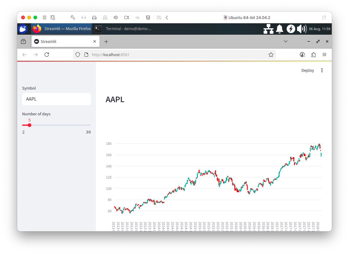
Figure 2-1. Streamlit.
On the web page, we can enter a new stock symbol in the text box and use the slider to change the number of days for TIME_BUCKET. Feel free to experiment with the code to suit your needs.
Summary
This chapter showed that SingleStore is a capable solution for working with time series data. Using the power of SQL and built-in functions, we achieved a great deal. SingleStore has extended its support for time series with the addition of FIRST, LAST and TIME_BUCKET.
Acknowledgements
I thank Dr John Pickford9 for advice and pointers to suitable time series datasets.
I am also grateful to Part Time Larry for his excellent video on Streamlit - Building Financial Dashboards with Python10 and the GitHub11 code for inspiring the Streamlit Visualization in this chapter.
-
https://martinfowler.com/bliki/PolyglotPersistence.html ↩
-
https://www.odbms.org/wp-content/uploads/2014/04/Multiple-Data-Models.pdf ↩
-
https://www.zdnet.com/article/the-nosql-database-glut-whats-the-real-price-of-the-current-boom/ ↩
-
https://www.techtarget.com/searchapparchitecture/tip/The-basics-of-polyglot-persistence-for-microservices-data ↩
-
https://www.kaggle.com/datasets/camnugent/sandp500 ↩
-
https://docs.singlestore.com/cloud/developer-resources/functional-extensions/analyzing-time-series-data/ ↩
-
https://en.wikipedia.org/wiki/Candlestick_chart ↩
-
https://docs.singlestore.com/cloud/developer-resources/functional-extensions/analyzing-time-series-data/ ↩
-
https://www.linkedin.com/in/john-pickford-50a9421/ ↩
-
https://www.youtube.com/watch?v=0ESc1bh3eIg ↩
-
https://github.com/hackingthemarkets/streamlit-dashboards ↩